You know what causal invariance is, right?
It’s, um, it’s when, well, causal invariance, something something something, right?
OK, so you might not know precisely what causal invariance is, but you do know that it’s a crucial concept in Wolfram Physics.
Causal invariance is how we get special relativity from the Wolfram model.
Causal invariance is how we get quantum mechanics from the Wolfram model.
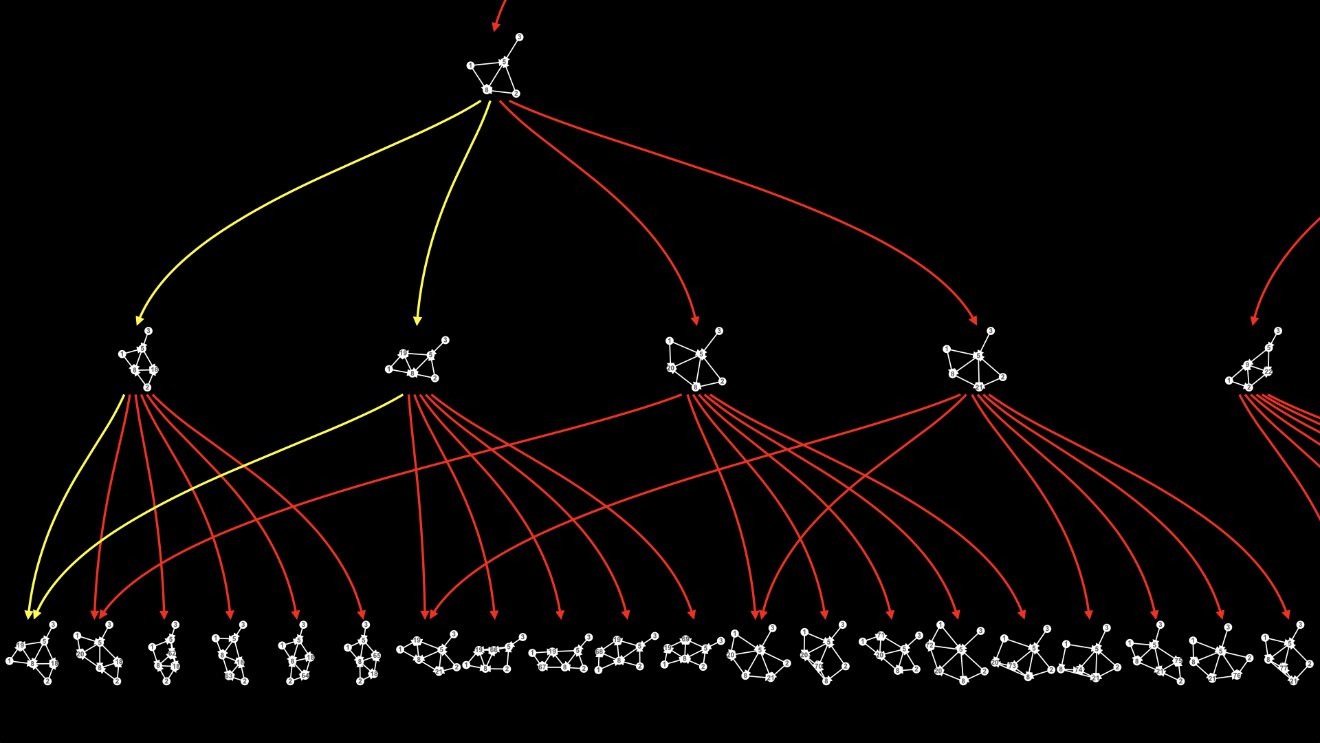
It’s going to take a few minutes, but I’m going to show you, in the multiway graph, precisely what causal invariance is.
—
I’ve shown you the multiway graph before, but if we’re going to be precise about causal invariance, we’re going to have to get much more precise about the multiway graph.
Remember, the multiway graph shows all possible evolutions of the universe through the application of a rule to the hypergraph.
I’m going to use the same rule I’ve used before, the one where you find two edges from the same node, delete one of those edges, and create a new edge from each of the three nodes to a new node.
Here’s the rule in action.
What I’m showing here is one way the universe might evolve under this rule. At every step, there’s more than one place in the hypergraph where I could apply the rule. So, at every step, I pick one of those places at random.
What the multiway graph shows, on the other hand, is every possible way the universe might evolve under the rule. When I’m drawing a multiway graph, at every step, I show how the universe evolves through every possible application of the rule.
Let’s start from the top.
History
Here are the first two levels of the multiway graph for this rule.
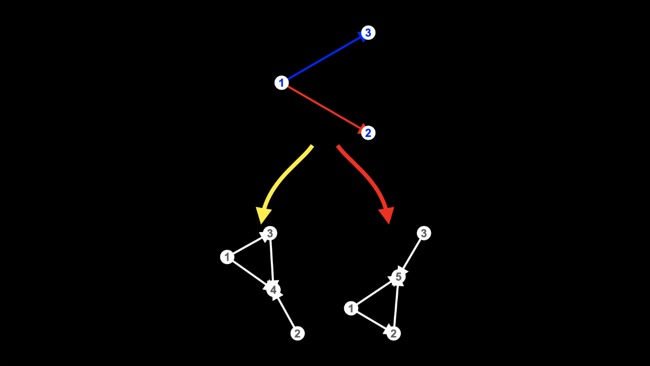
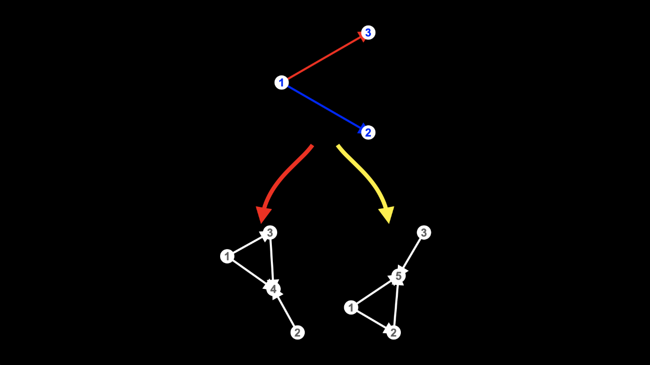
Starting from the hypergraph at the top, there are two possible ways we could apply the rule.
It’s easy enough to find two edges from the same node. That’s all the hypergraph at the top is: two edges from the same node.
But when it comes to deleting one of those two edges, we have a choice to make. We could delete either the bottom edge, from node 1 to node 2, or the top edge, from node 1 to node 3.
Choosing to delete the bottom edge gives the hypergraph on the left:
Choosing to delete the top edge gives the hypergraph on the right.
These two hypergraphs look kinda similar, but they’re not exactly the same:
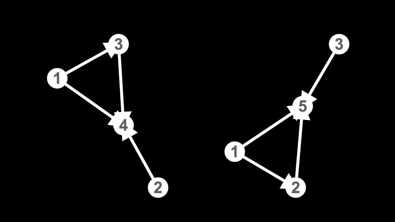
In the one on the left, node 2, for example, is connected by a single edge to the new node, but in the one on the right, node 2 is still connected by an edge from node 1, as well as by the edge to the new node.
And you can see that I’ve labelled the new node differently in the two different hypergraphs: it’s labelled node 4 in the one on the left but node 5 in the one on the right.
How we label the nodes is going to be crucial in determining when two universes are different and when they’re the same.
The reason I’ve labelled the new nodes differently is that they have different histories.
The new node 4 in the hypergraph on the left was created through the application of the rule to the edges {1, 2} and {1, 3}, where it’s the first edge, {1, 2}, that’s deleted.

The new node 5 in the hypergraph on the right, however, was created through the application of the rule to the edges {1, 3} and {1, 2} ... the same edges, but because they’re the other way around, it’s the first edge, {1, 3}, that’s deleted.

If a node is created through the application of the rule to the same edges in the same order, then I’ll give that node the same label, no matter where in the multiway graph it appears.
But if, as in this case, nodes are created through the application of the rule to different edges, or to the same edges in a different order, then I’ll give those nodes different labels.
In other words, nodes are identified by their histories:
- nodes in different branches of the multiway graph with the same history are the same node;
- nodes in different branches of the multiway graph with different histories are different nodes.
Let’s go deeper into the multiway graph, and you’ll see why this matters.
Deeper still and deeper
So, after applying the rule once, we have two hypergraphs:
There are two ways the rule can be applied to each of these two hypergraphs.
So, at the next level of the multiway graph, we have four hypergraphs:
And there are four ways the rule can be applied to each of these four hypergraphs.
So, at the next level of the multiway graph, we have sixteen hypergraphs:
Let’s take a closer look at a few of these paths through the multiway graph, in other words, at a few of these possible evolutions of the universe.
You can see how there are four ways the rule can be applied to this hypergraph:

Remember, to apply the rule, we need to find two edges from the same node.
Well, there are two edges from node 1, one to node 5 and another to node 8:
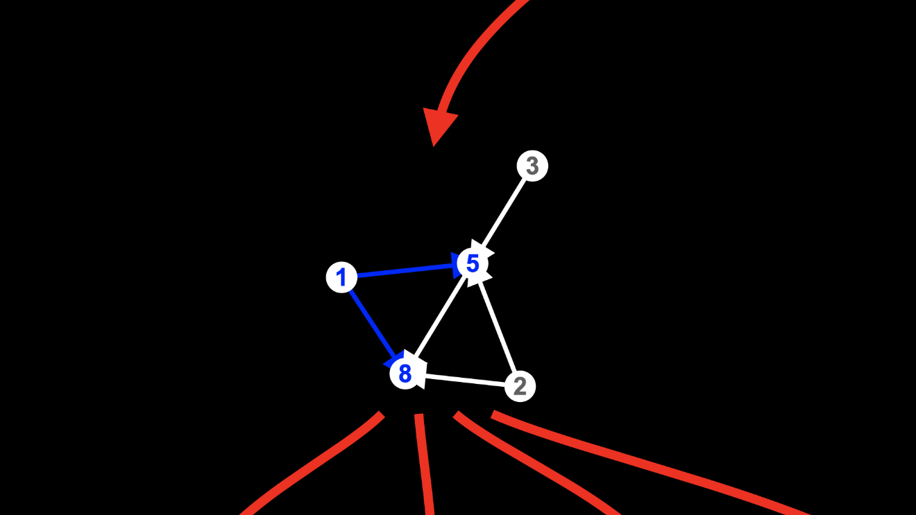
And there are two edges from node 2, again, one to node 5 and another to node 8:
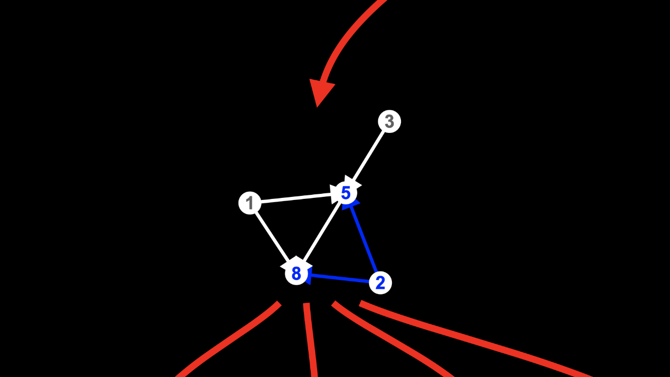
In each of those two cases, there are two possible ways I could apply the rule.
If we match the two edges from node 1, we could delete either the edge to node 5:
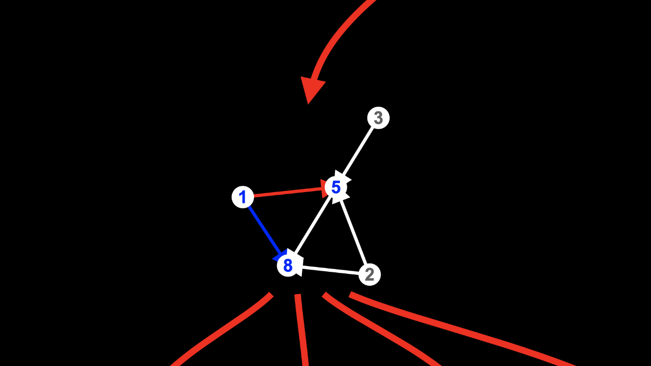
or the edge to node 8:
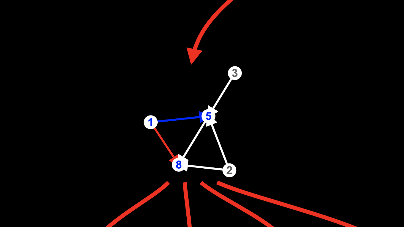
And if we match the two edges from node 2, again, we could delete either the edge to node 5:
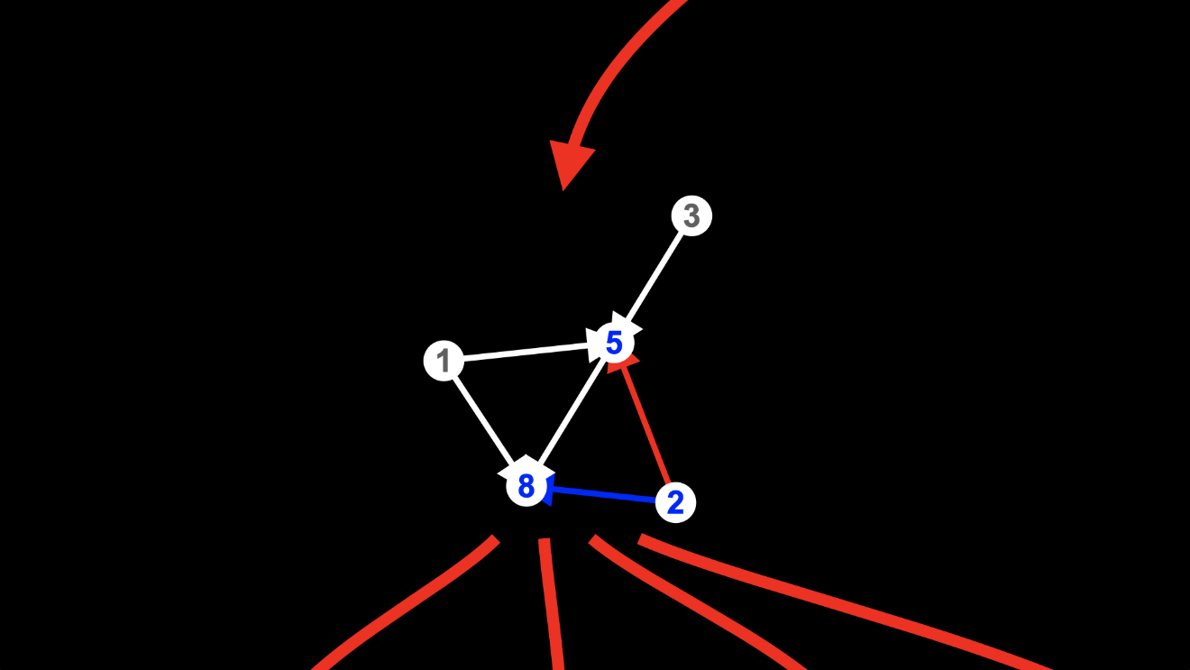
or the edge to node 8:

That’s how this hypergraph evolves into any of four different hypergraphs at the next level of the multiway graph:
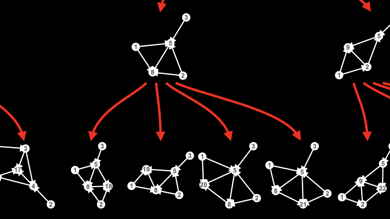
In each of these four cases, the new node created by the rule has a different history.
That’s why I give these new nodes different labels: 18, 19, 20 and 21.
So, there’s a lot of branching in these first few levels of the multiway graph:
You might imagine that if we go one level deeper, we’ll see a whole lot more branching.
And we do.
But we see something else, too, something that’s the opposite of branching, something that makes the hypergraph a viable model of our universe.
What we see is some of these branches coming back together.
Let’s come together
Here’s the multiway graph one level deeper:
There’s a lot going on here, but you can see that some of the branches formed when we applied the rule a third time come back together when we apply the rule a fourth time:
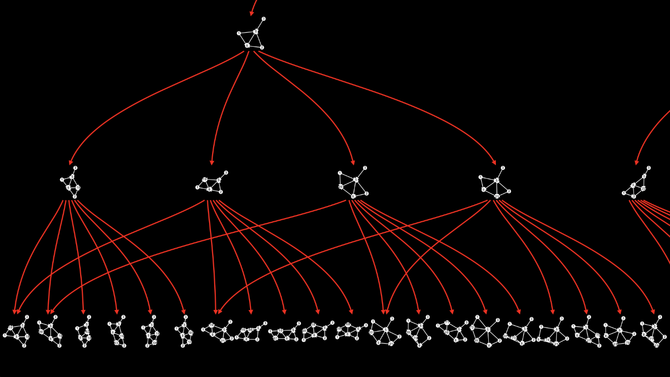
Let’s take a closer look at one of those branches.
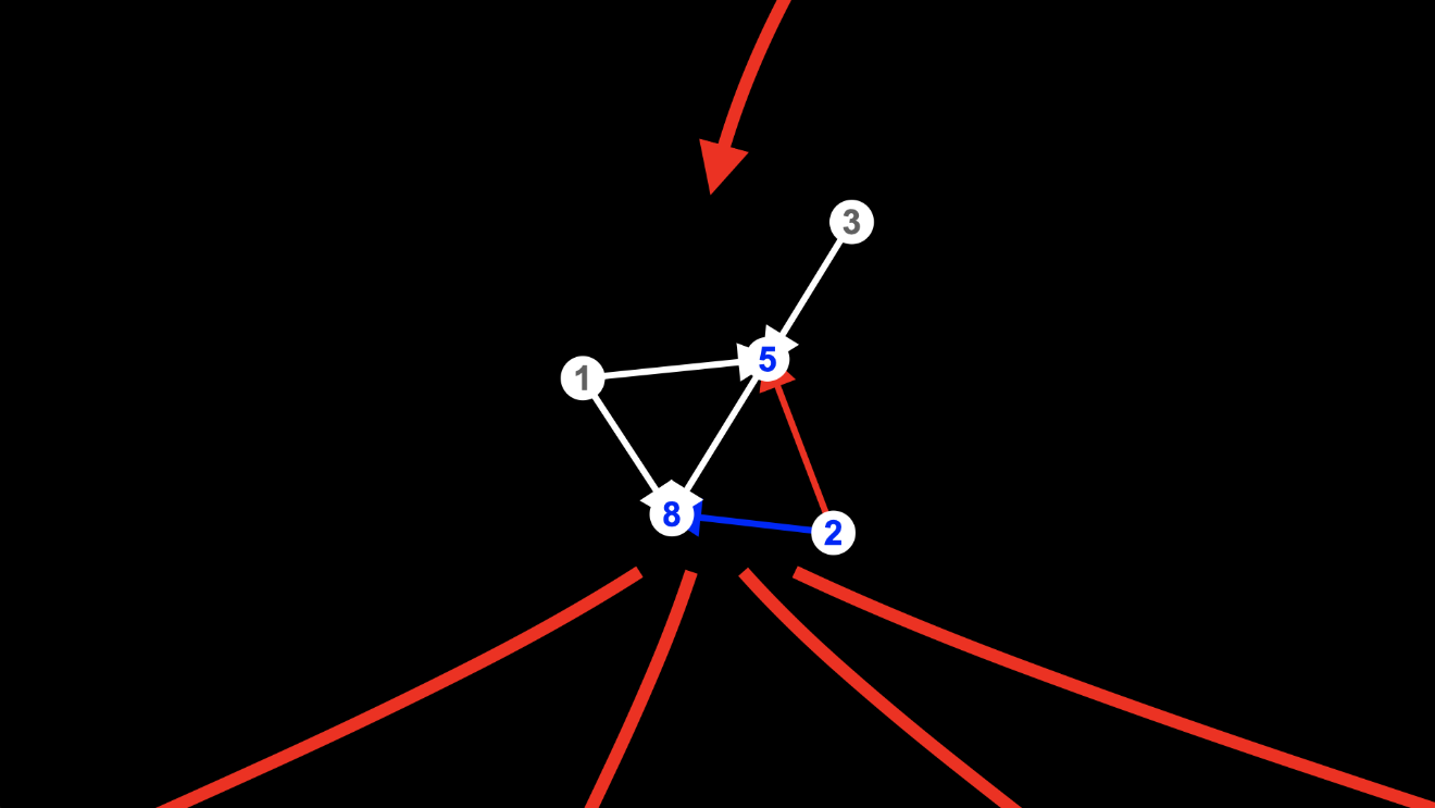
We’ve already seen what happened when these two hypergraphs were created, the ones in which nodes 18 and 19 appeared for the first time:
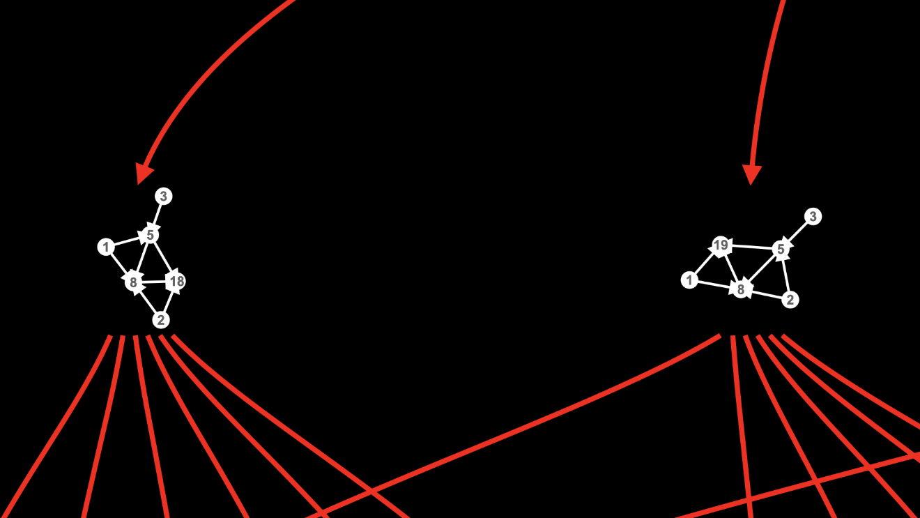
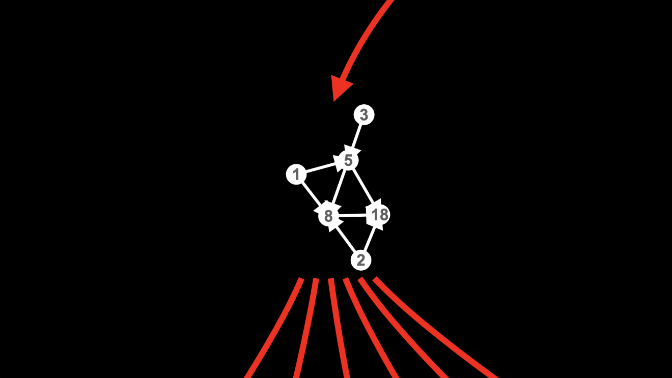
To arrive at the hypergraph on the left, we applied the rule to the two edges from node 2, deleting the one from node 2 to node 5:
and creating the new node 18:
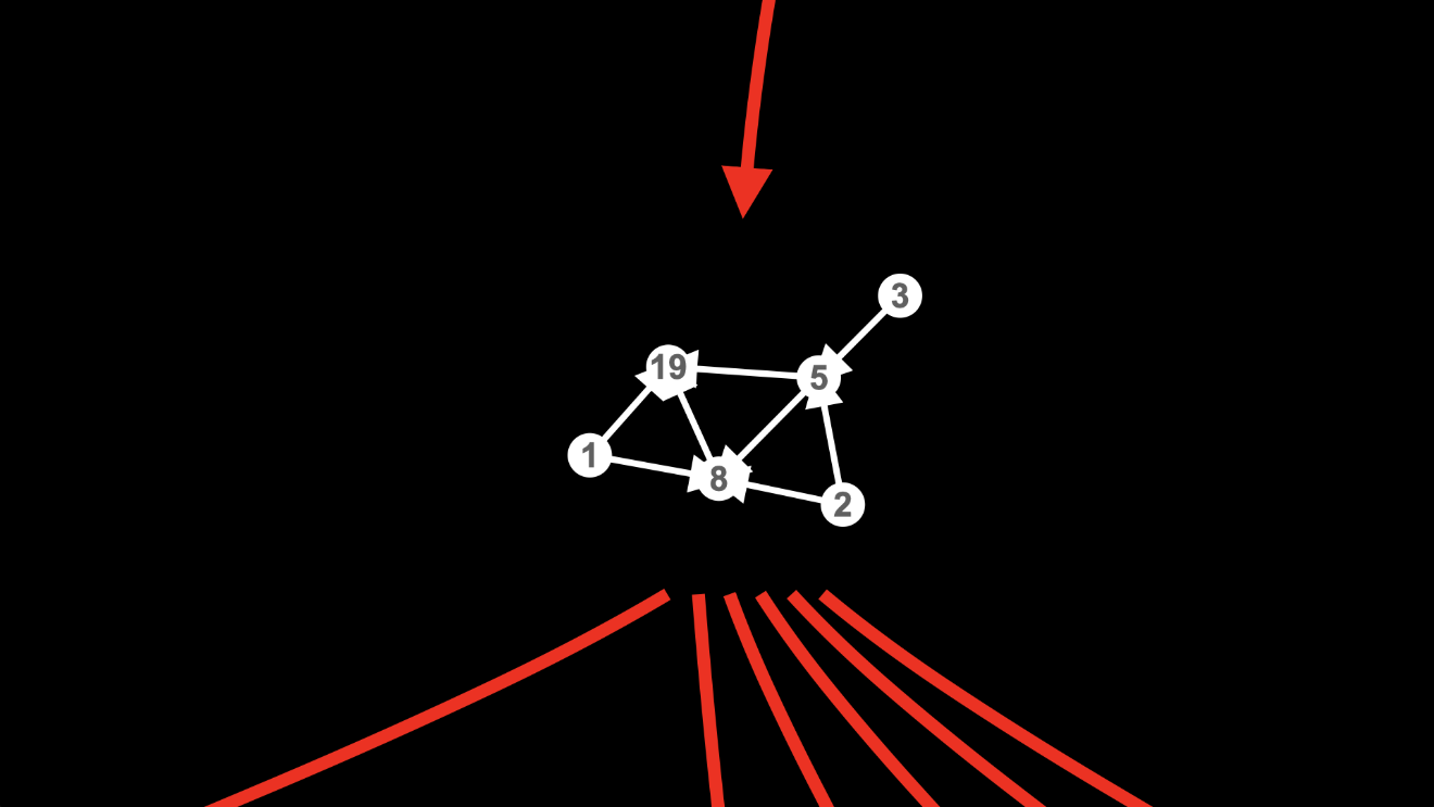
And to arrive at the hypergraph on the right, we applied the rule to the two edges from node 1, deleting the one from node 1 to node 5:
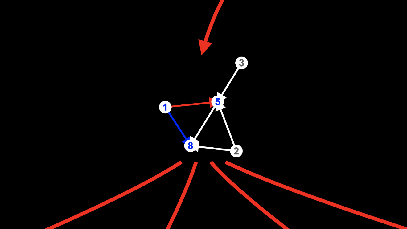
and creating the new node 19:
The thing is, neither of these applications of the rule prevents us from performing the other application of the rule at the next step.
Deleting the edge from node 2 to node 5 leaves the edges from node 1 to nodes 5 and 8 intact, ready to be matched at the next step:
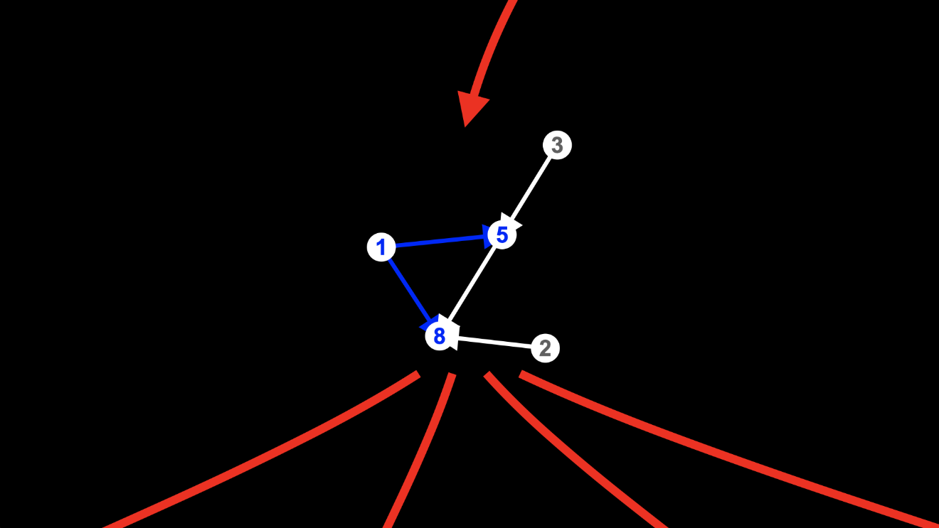
And deleting the edge from node 1 to node 5 leaves the edges from node 2 to nodes 5 and 8 intact, again, ready to be matched at the next step:
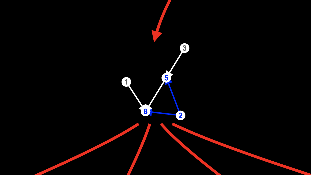
It doesn’t matter which order we do it in.
We can match the edges from node 2 and create the new node 18 first, then match the edges from node 1 and create the new node 19.
Or we can match the edges from node 1 and create the new node 19 first, then match the edges from node 2 and create the new node 18.
Either way...

...we end up with this hypergraph:
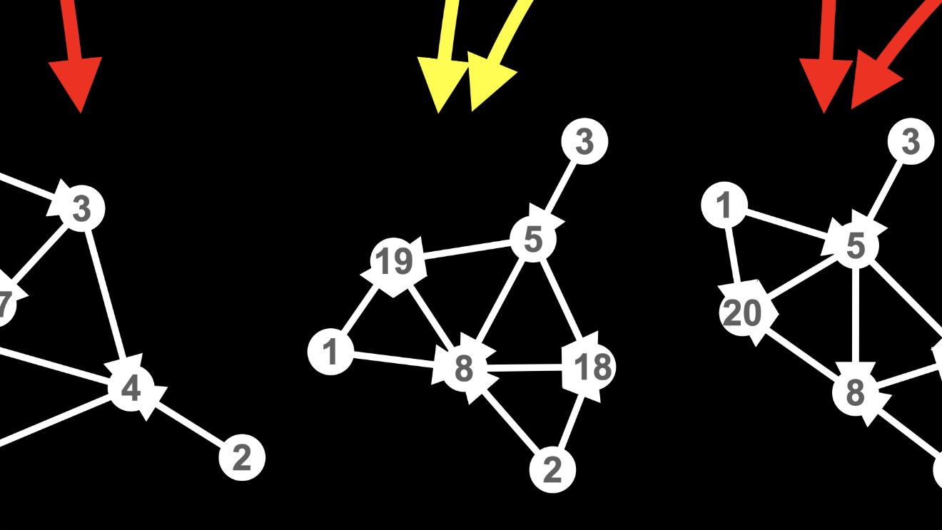
The branches in the multiway graph created when we applied the rule a third time come back together when we apply the rule a fourth time.
You can see that my labelling the nodes according to their histories is crucial in recognizing this coming back together of the branches.
It doesn’t matter which path we take through the multiway graph, node 18 is still node 18, since it was created through the application of the rule to the edges {2, 5} and {2, 8}, and node 19 is still node 19, since it was created through the application of the rule to the edges {1, 5} and {1, 8}.
On the other side of the world
It’s not surprising, when you think about it, that it sometimes doesn’t matter which order we do things in.
Imagine a much larger hypergraph than the ones I’ve been showing you, representing a much larger universe. You know, like our own.
Imagine applying the rule to some edges on one side of the universe:
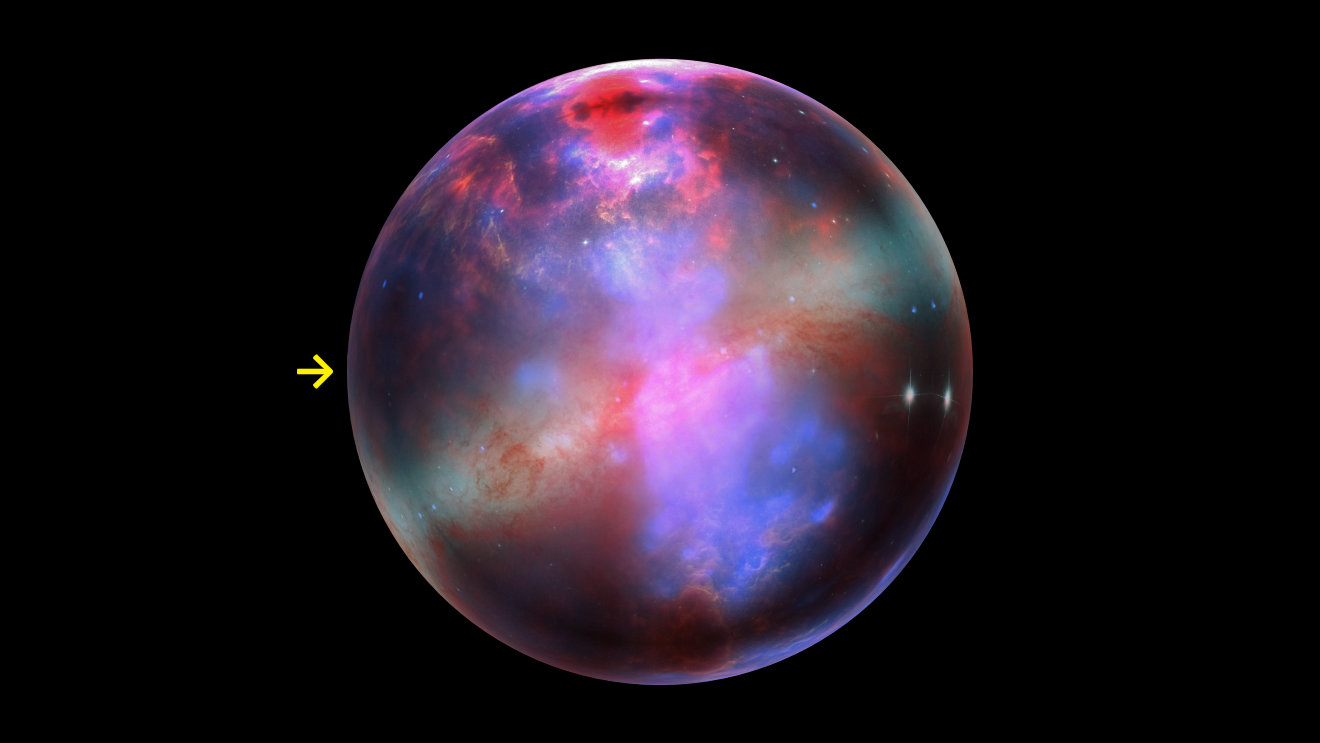
then to some edges on the other side of the universe:

Now imagine doing it the other way around, first applying the rule to the edges on the other side of the universe:
then applying it to the edges on the original side of the universe:

How’s it going to matter which way around we do it?
Who’s even going to notice?
What experiment could we possibly perform that’d distinguish between a universe in which these applications of the rule happened in one order and a universe in which they happened in the other order?
When the branches come back together, the world we find ourselves in having followed one branch is the same as the world we find ourselves in having following the other branch.
This changes everything
It’s difficult to overstate the importance of this coming back together of the branches for Wolfram Physics.
Indeed, it’s difficult to overstate the importance of this coming back together of the branches for the universe.
The idea of a branching universe isn’t new in physics.
In the many worlds interpretation of quantum mechanics, the universe is forever branching and branching and branching.
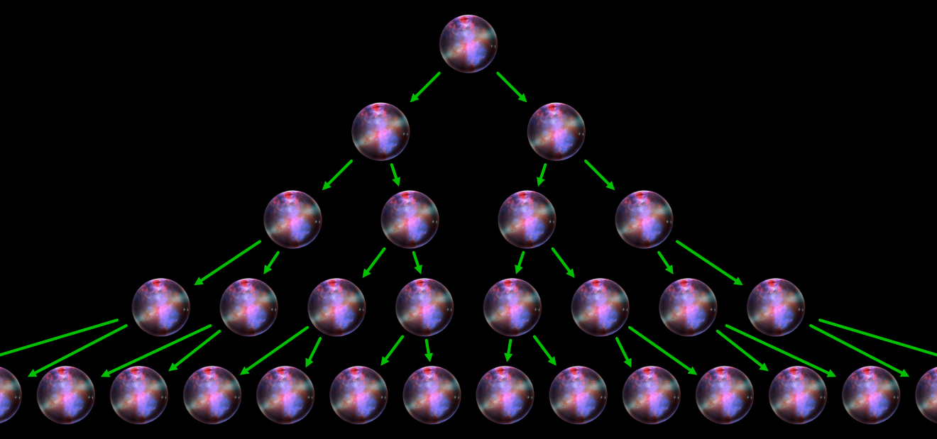
I’ve always thought of the many worlds interpretation as a provocative visualization, but not a scientific theory. After all, if these countless different branches of the universe remain forever separate – if no branch can have any influence on any other branch – then the many worlds interpretation is unfalsifiable. We’ll never be able to make contact with any branch of the universe other than our own, so we’ll never be able to prove that these other worlds exist, and we’ll never be able to prove these other worlds don’t exist.
But if the branches can come back together, well, that changes everything.
Suddenly there’s the promise that quantum mechanics might be transformed: from a theory in which there’s no way to choose between the countless possible branches of the universe, except randomly; to a theory in which there might be a way to collapse multiple paths through the multiway graph to a single, objective reality.
What is causal invariance?
OK, let’s bring this home.
What is causal invariance?
Well, loosely...
Causal invariance is different branches of the multiway graph coming back together.

But I promised to tell you precisely what causal invariance is.
Precisely, then...
If, for a particular rule, whenever there’s a two-way branch in the multiway graph, there exist paths through the multiway graph along which the two branches come back together, then the rule is causally invariant.
The two branches might not come back together immediately, as they did in the case I just showed you. Indeed, it might be many, many levels deeper into the multiway graph that they come back together.
And there may be other paths through the multiway graph along which the two branches don’t come back together. Indeed, in the case I just showed you, I carefully picked out a path along which the branches do come back together...

...and studiously ignored all the other paths along which they don’t come back together...
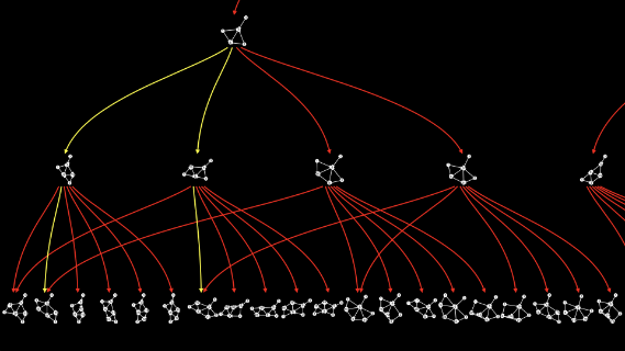
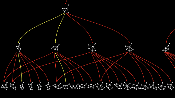
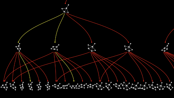
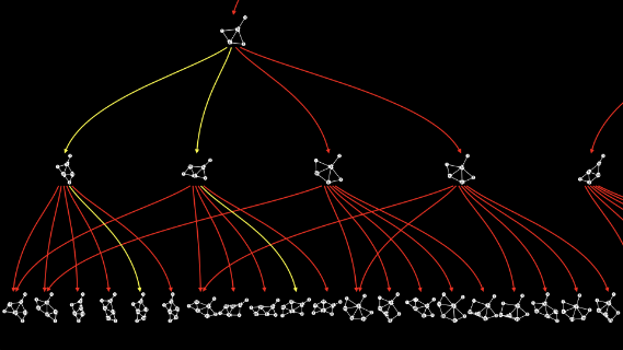
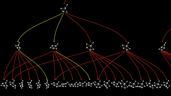
...at least, not immediately.
But as long as, whenever there’s a two-way branch, there exist paths along which the two branches come back together, then that’s causal invariance.
What is causality?
In this article, I’ve barely scratched the surface of causal invariance and its implications.
I’ll have much more to say about it in future articles.
But before we go any further, I want to acknowledge that I’ve thrown in a contentious word, without saying what I mean by it.
That word is “causal”.
Why do we call the coming back together of branches in the multiway graph “causal” invariance?
What is causality?
If you think you know the answer to this seemingly simple question, then my next article might make you think again.